Art + #rstats
Sharla Gelfand
Toronto Data Workshop
1 / 41
why aRt?
3 / 41
4 / 41
5 / 41
You can do both
Digital art is fast, iterative, surprising
Less "I suck at this" beginner hurdles
Less startup cost
I ❤️ R
6 / 41
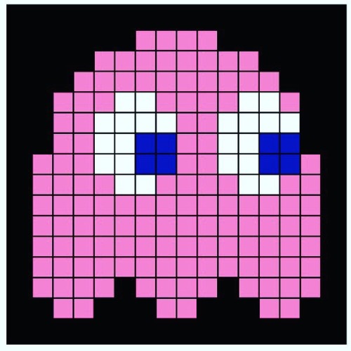
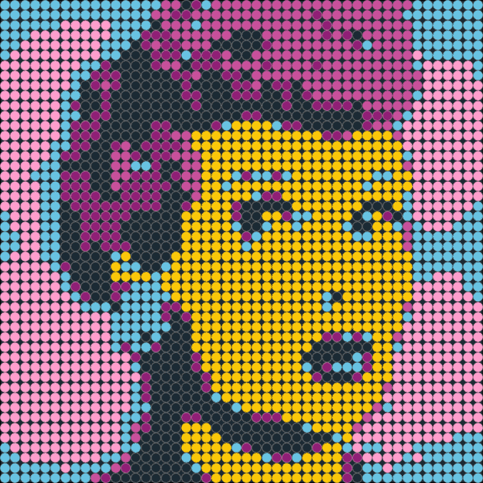
Pixel Art
A form of digital art where images are edited at the pixel level.
Think 8-bit video games aesthetics.
7 / 41
library(ggplot2)library(dplyr)smile <- expand.grid(x = 1:8, y = 1:8) %>% filter(!(x %in% c(1, max(x)) & y %in% c(1, max(y)))) %>% filter(!(x %in% c(2, max(x) - 1) & y %in% c(1, max(y)))) %>% filter(!(x %in% c(1, max(x)) & y %in% c(2, max(y) - 1)))ggplot() + geom_tile( data = smile, aes(x = x, y = y), width = 1, height = 1, size = 1, fill = "yellow", colour = "black" ) + coord_equal() + theme_void()9 / 41
library(ggplot2)library(dplyr)smile <- expand.grid(x = 1:8, y = 1:8) %>% filter(!(x %in% c(1, max(x)) & y %in% c(1, max(y)))) %>% filter(!(x %in% c(2, max(x) - 1) & y %in% c(1, max(y)))) %>% filter(!(x %in% c(1, max(x)) & y %in% c(2, max(y) - 1)))ggplot() + geom_tile( data = smile, aes(x = x, y = y), width = 1, height = 1, size = 1, fill = "yellow", colour = "black" ) + coord_equal() + theme_void()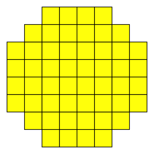
9 / 41
library(ggplot2)library(dplyr)smile <- expand.grid(x = 1:8, y = 1:8) %>% filter(!(x %in% c(1, max(x)) & y %in% c(1, max(y)))) %>% filter(!(x %in% c(2, max(x) - 1) & y %in% c(1, max(y)))) %>% filter(!(x %in% c(1, max(x)) & y %in% c(2, max(y) - 1)))eyes <- data.frame(x = c(3, 6), y = c(6, 6))ggplot() + geom_tile( data = smile, aes(x = x, y = y), width = 1, height = 1, size = 1, fill = "yellow", colour = "black" ) + geom_tile( data = eyes, aes(x = x, y = y), width = 1, height = 1, fill = "black", colour = "black" ) + coord_equal() + theme_void()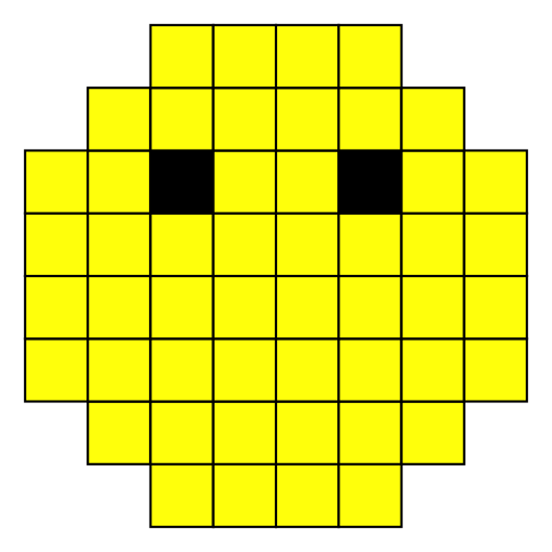
10 / 41
library(ggplot2)library(dplyr)smile <- expand.grid(x = 1:8, y = 1:8) %>% filter(!(x %in% c(1, max(x)) & y %in% c(1, max(y)))) %>% filter(!(x %in% c(2, max(x) - 1) & y %in% c(1, max(y)))) %>% filter(!(x %in% c(1, max(x)) & y %in% c(2, max(y) - 1)))eyes <- data.frame(x = c(3, 6), y = c(6, 6))mouth <- data.frame(x = 3:6, y = c(3, 2, 2, 3))ggplot() + geom_tile( data = smile, aes(x = x, y = y), width = 1, height = 1, size = 1, fill = "yellow", colour = "black" ) + geom_tile( data = eyes, aes(x = x, y = y), width = 1, height = 1, fill = "black", colour = "black" ) + geom_tile( data = mouth, aes(x = x, y = y), width = 1, height = 1, fill = "black", colour = "black" ) + coord_equal() + theme_void()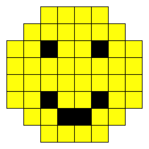

11 / 41
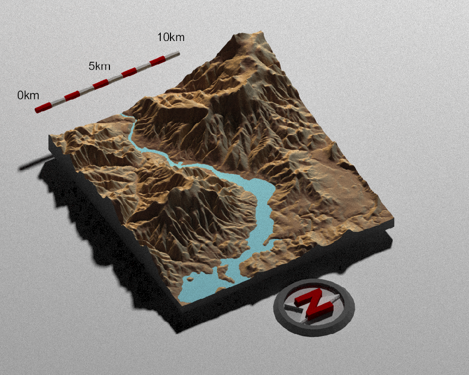
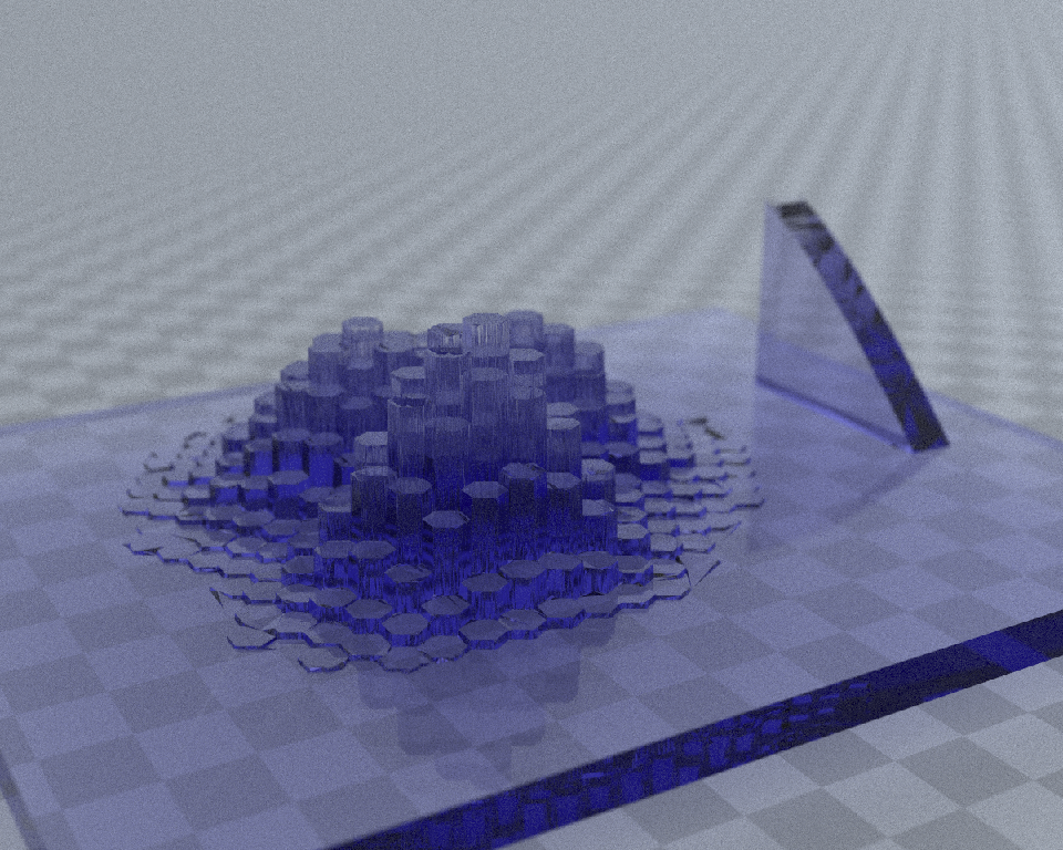
Rendering
Recreating an image (realistic or not) from a 2D or 3D model, via a computer program.
12 / 41
library(rayrender)generate_ground( material = diffuse(color = "#dd99ba") ) %>% render_scene()16 / 41
library(rayrender)generate_ground( material = diffuse(color = "#dd99ba") ) %>% render_scene()16 / 41
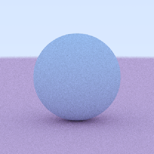
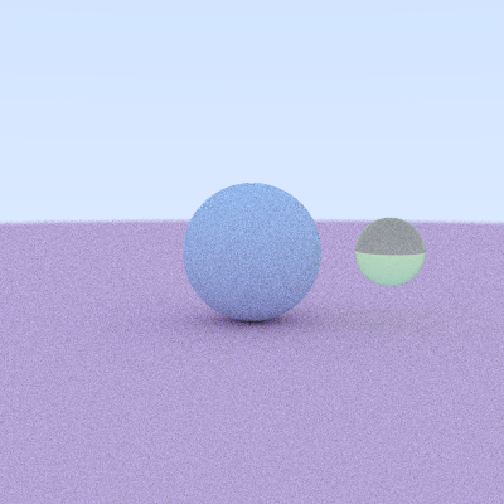
library(rayrender)generate_ground( material = diffuse(color = "#dd99ba") ) %>% add_object(sphere( material = diffuse(color = "#99badd") )) %>% render_scene()17 / 41
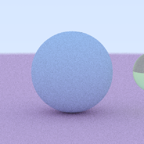
library(rayrender)generate_ground( material = diffuse(color = "#dd99ba") ) %>% add_object(sphere( material = diffuse(color = "#99badd") )) %>% add_object(sphere( x = 2, radius = 0.5, material = dielectric(color = "#badd99") )) %>% render_scene( )18 / 41
library(rayrender)generate_ground( material = diffuse(color = "#dd99ba") ) %>% add_object(sphere( material = diffuse(color = "#99badd") )) %>% add_object(sphere( x = 2, radius = 0.5, material = dielectric(color = "#badd99" )) %>% render_scene( fov = 40 )19 / 41
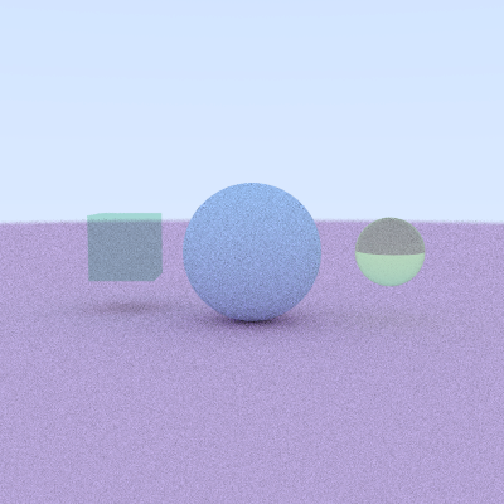
library(rayrender)generate_ground( material = diffuse(color = "#dd99ba") ) %>% add_object(sphere( material = diffuse(color = "#99badd") )) %>% add_object(sphere( x = 2, radius = 0.5, material = dielectric(color = "#badd99") )) %>% add_object(cube( x = -2, z = -1, width = 1, material = metal(color = "#99ddba") )) %>% render_scene( fov = 40 )20 / 41
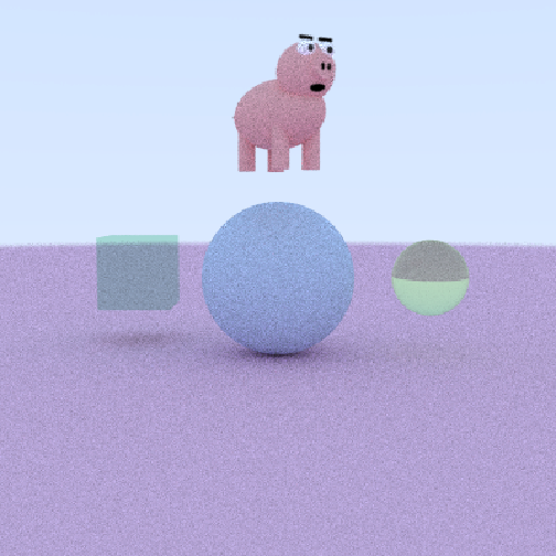
library(rayrender)generate_ground( material = diffuse(color = "#dd99ba") ) %>% add_object(sphere( material = diffuse(color = "#99badd") )) %>% add_object(sphere( x = 2, radius = 0.5, material = dielectric(color = "#badd99") )) %>% add_object(cube( x = -2, z = -1, width = 1, material = metal(color = "#99ddba") )) %>% add_object(pig( y = 1, z = 1, scale = 0.4, angle = c(0, -60, 0) )) %>% render_scene( fov = 40 )21 / 41
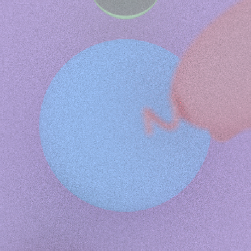
library(rayrender)generate_ground( material = diffuse(color = "#dd99ba") ) %>% add_object(sphere( material = diffuse(color = "#99badd") )) %>% add_object(sphere( x = 2, radius = 0.5, material = dielectric(color = "#badd99") )) %>% add_object(cube( x = -2, z = -1, width = 1, material = metal(color = "#99ddba") )) %>% add_object(pig( y = 1, z = 1, scale = 0.4, angle = c(0, -60, 0) )) %>% render_scene( fov = 40, lookfrom = c(-1, 4, 0) )22 / 41
Generative art
"Generative art is art programmed using a computer that intentionally introduces randomness as part of its creation process."
- Why Love Generative Art?
23 / 41
Generative art
The environment is constrained, but decisions are made randomly, rather than by the artist.
library(ggplot2)library(ggforce)n <- 5ggplot() + geom_circle(aes( x0 = rnorm(n), y0 = rnorm(n), r = runif(n) )) + theme_void()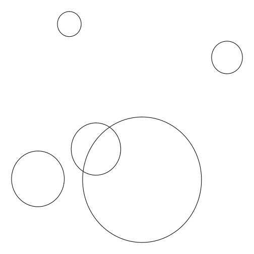
25 / 41
Generative art
Additional complexity doesn't mean additional time or effort.
library(ggplot2)library(ggforce)n <- 100ggplot() + geom_circle(aes( x0 = rnorm(n), y0 = rnorm(n), r = runif(n) )) + theme_void()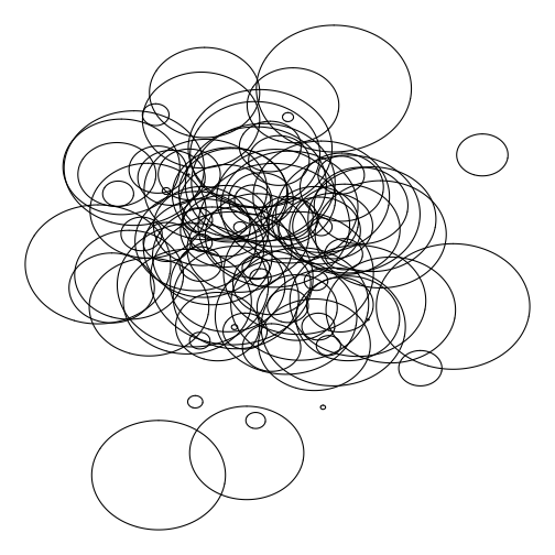
26 / 41
generativeart package
library(generativeart)formula <- list( x = quote(rnorm(5) * x_i - cos(y_i^2)), y = quote(rnorm(5) * y_i^2 + sin(x_i)))generate_img( formula = formula, polar = FALSE, nr_of_img = 1)27 / 41
generativeart package
library(generativeart)formula <- list( x = quote(rnorm(5) * x_i - cos(y_i^2)), y = quote(rnorm(5) * y_i^2 + sin(x_i)))generate_img( formula = formula, polar = FALSE, nr_of_img = 1)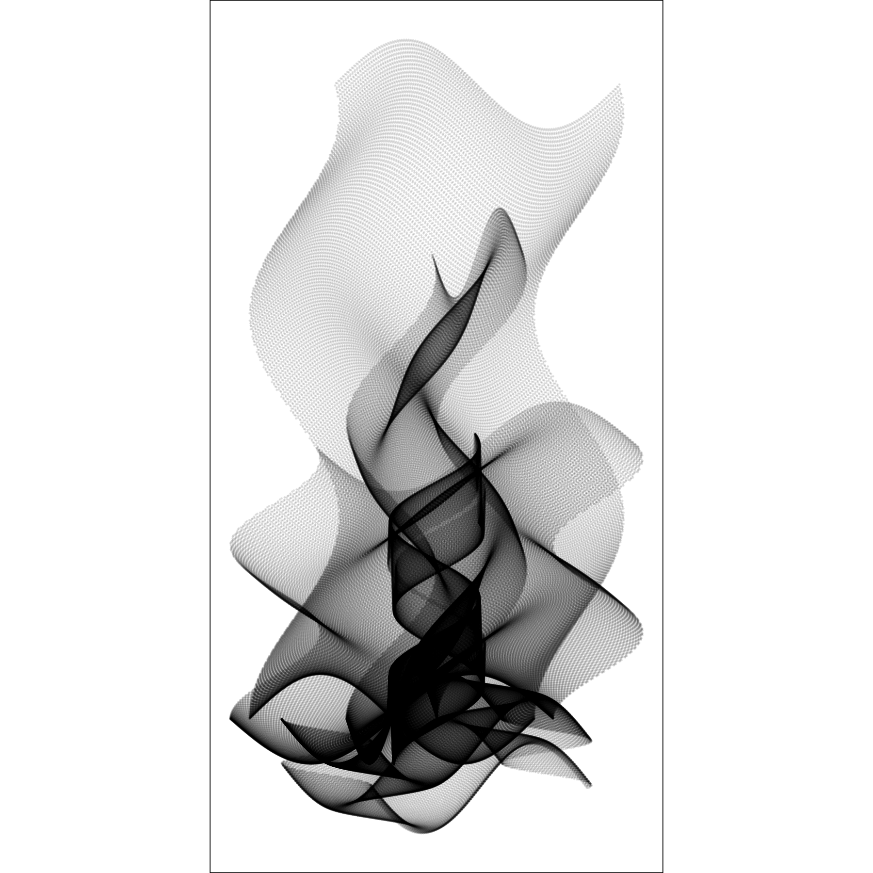
27 / 41
generativeart package
library(generativeart)formula <- list( x = quote(rnorm(5) * x_i - cos(y_i^2)), y = quote(rnorm(5) * y_i^2 + sin(x_i)))generate_img( formula = formula, polar = TRUE, nr_of_img = 2)Seed: 2917
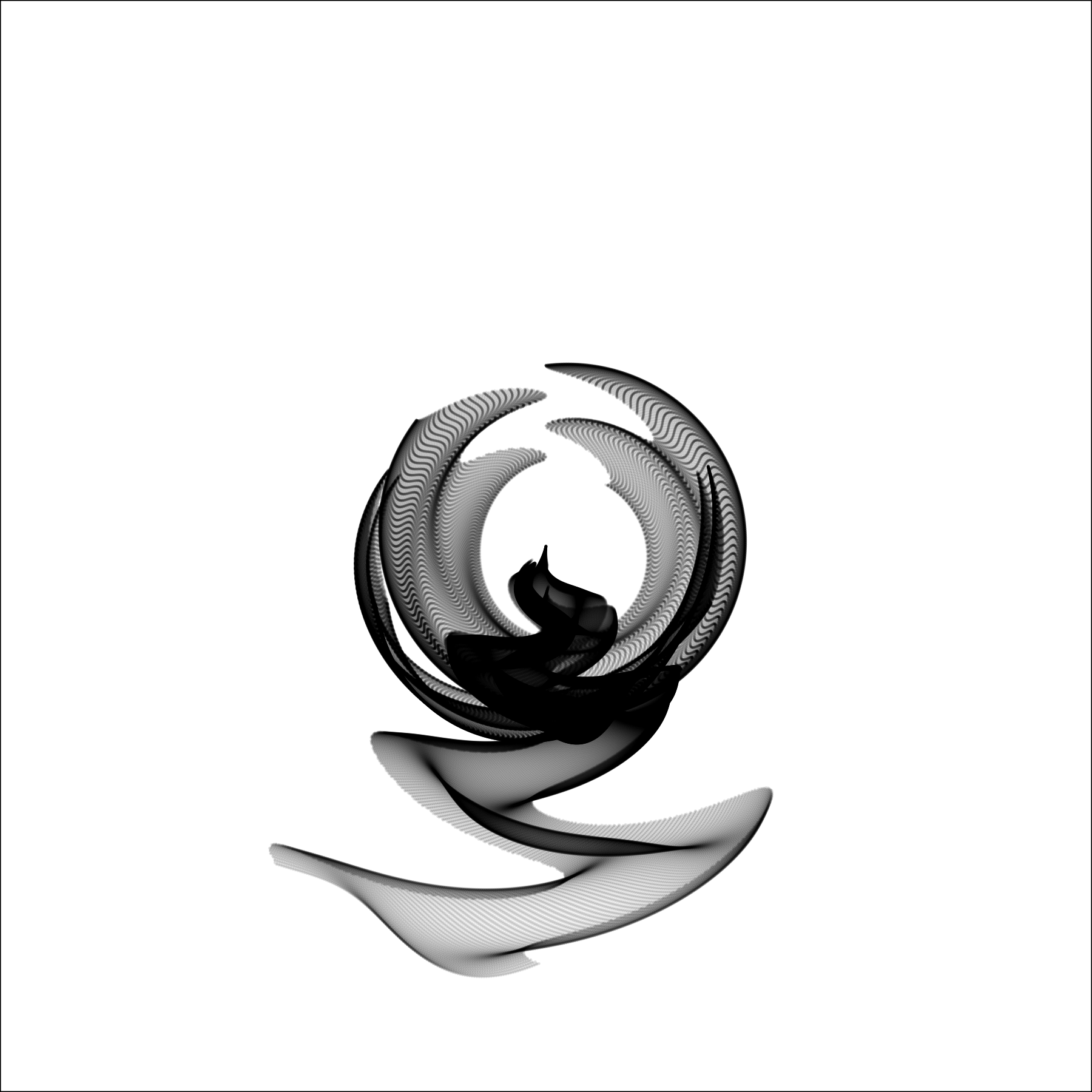
28 / 41
generativeart package
library(generativeart)formula <- list( x = quote(rnorm(5) * x_i - cos(y_i^2)), y = quote(rnorm(5) * y_i^2 + sin(x_i)))generate_img( formula = formula, polar = TRUE, nr_of_img = 2)Seed: 3553
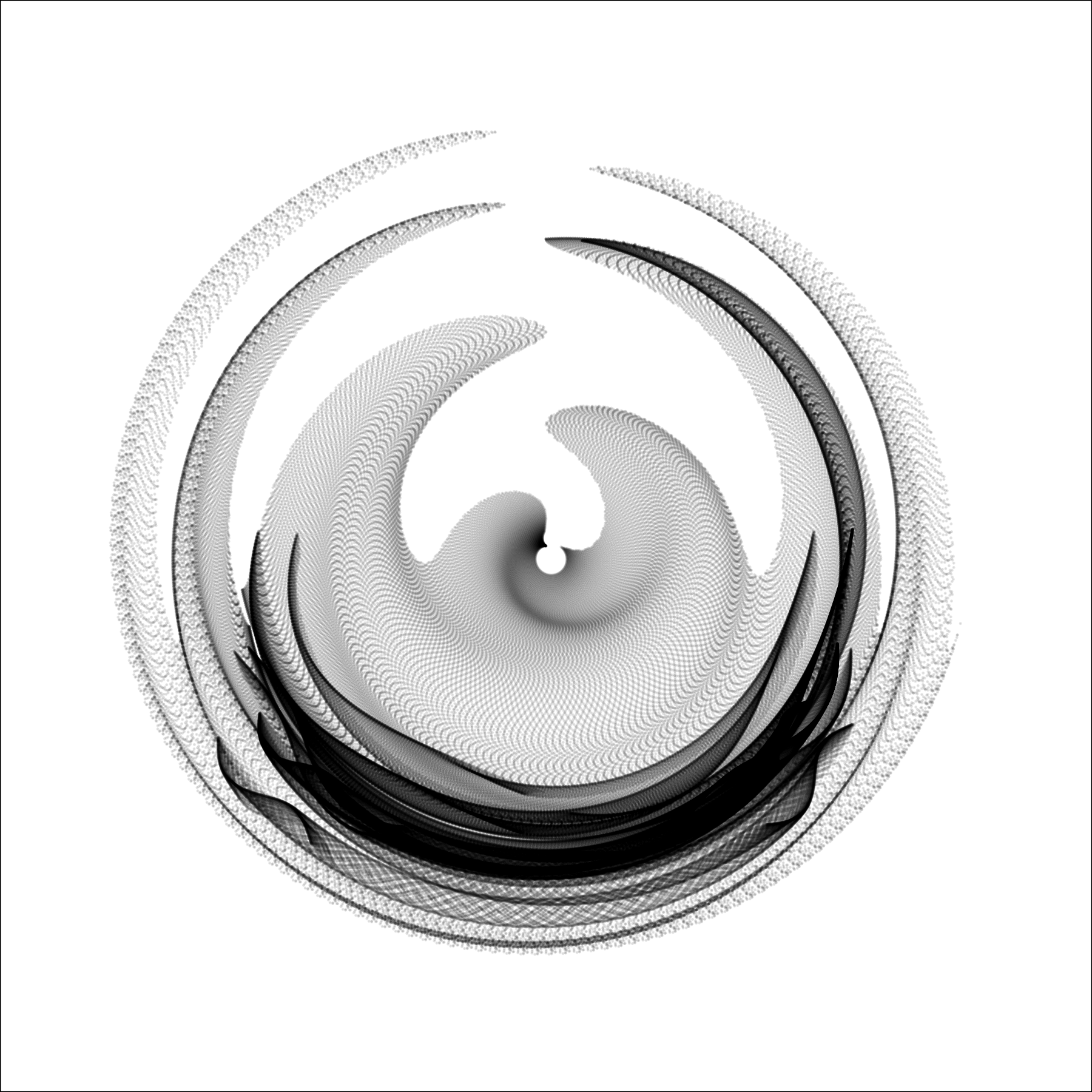
29 / 41
generativeart package
library(generativeart)formula <- list( x = quote(runif(5) * x_i - cos(y_i^2)), y = quote(rnorm(5) * y_i^2 + sin(x_i)))generate_img( formula = formula, polar = TRUE, nr_of_img = 1, color = "red")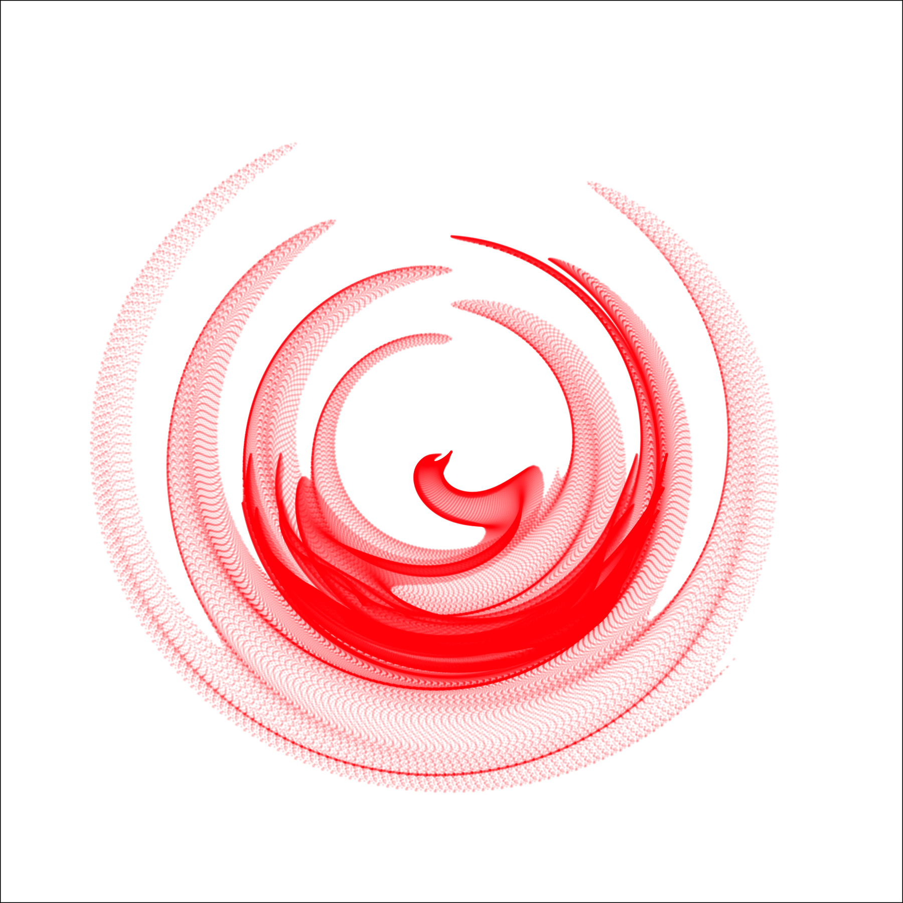
30 / 41
flametree package
library(flametree)flametree_grow( seed = 1234, time = 1, split = 2) %>% flametree_plot()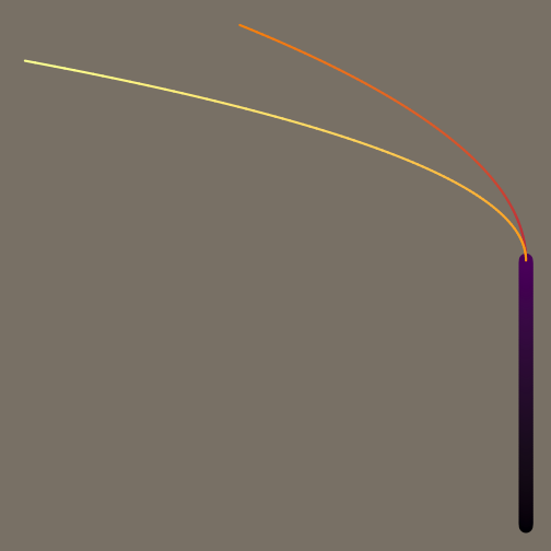
31 / 41
flametree package
library(flametree)flametree_grow( seed = 1234, time = 2, split = 2) %>% flametree_plot()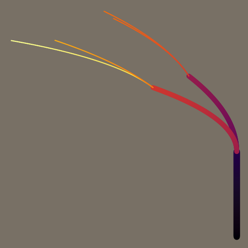
32 / 41
flametree package
library(flametree)flametree_grow( seed = 1234, time = 2, split = 4) %>% flametree_plot()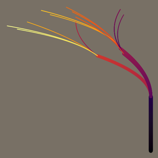
33 / 41
flametree package
library(flametree)flametree_grow( seed = 1234, time = 5, split = 4 ) %>% flametree_plot( background = "pink", palette = "ggthemes::Classic Red-Green Light")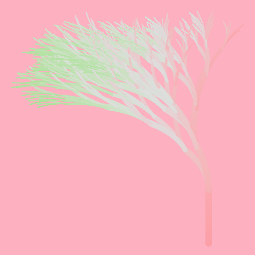
34 / 41
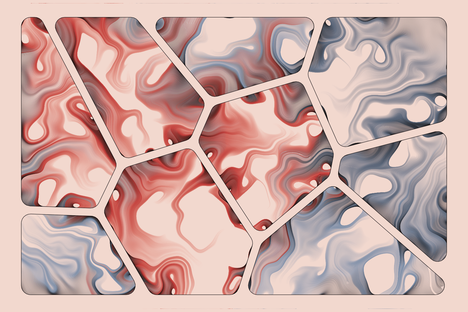
"For me, the sweet spot of generative art lies in creating a system that you know well enough to set it up for success, but is so complex that you still get surprised when you see the result."
35 / 41
And more!
36 / 41
